
Using examples from: The Algorithmic Beauty of Plants: http://algorithmicbotany.org/papers/abop/abop.pdf
Contents
- Contents
- Turtle sequence
- Line Drawing Commands
- Rotation Commands
- Adding incremental changes (eg. per generation)
- Geometry Commands
- Variables representing Values
- Behavioural Commands
- Branching
- Edge Rewrite
- Node Rewrite
- Branching Structures
- Symbol variables
- Control variables over time
- Usage in a branching tree:
- Using Custom Values
- Monopodial Tree
- Sympodial Tree
- Gravity (tropism)
- Ternary Tree
- Input Geometry in L-Systems
- Stamping Geometry
- Example using stamp expression to choose geometry
- Example using stamp expression to change colour
- Probability
- Conditionals
- Bringing together Geometry Inputs, Custom Variables and Conditionals
- Context Sensitive L-Systems
- Phyllotaxis
- Sunflower
- Creating Leaves from Surface Geometry
- Cordate Leaf
- A family of simple leaves
- A Rose Leaf
- Ferns and other Compound Leaves
- Compound leaves with alternating branching patterns
To see the full turtle sequence being generated by an L-System open up an HScript Textport (alt+shift+t) And type: opinfo /pathto/L-SystemYou can drag the L-System node into the textport to get the path automatically. |
Turtle sequence
The basic L-system commands are used to draw a line or series of lines. Each command follows on from the last, so as to draw a line through space. It helps to imagine a point (or turtle) moving forwards, and rotating left, right, pitching up and down, and rolling about its axis.
Line Drawing Commands
| F | Move forward a step, drawing a line connecting the previous position to the new position. |
| f | Move forward without drawing. |
| H | Move forward half a step, drawing a line connecting the previous position to the new position. |
| h | Move forward half a step without drawing.. |
| G | Move forward but don’t record a vertex distance |
| Without further information the above commands use the Value ‘step size’ for length | |
| F(l,w,s,d) f(l,w,s,d) etc | For each of the above commands (l,s,w,d) assigns distance l of width w using s cross sections of d divisions each. |
| Not all of these values need to be set eg. | |
| F(l) | creates a line of distance (length) l |
| F(l,w) | Creates a line of distance l and width w |
Rotation Commands
| + | Turn right a degrees. |
| – | Turn left a degrees (minus sign). |
| & | Pitch up a degrees. |
| ^ | Pitch down a degrees. |
| \ | Roll clockwise a degrees. |
| / | Roll counter-clockwise a degrees. |
| | | Turn 180 degrees |
| * | Roll 180 degrees |
| ~(a) | Pitch / Roll / Turn random amount up to a given number of degrees (a) . Default 180. |
| $(x,y,z) | Rotates the turtle so the up vector is (0,1,0). Points the turtle in the direction of the point (x,y,z). Default behavior is only to orient and not to change the direction. |
| Without further information these commands use the Value ‘Angle’ to determine the angle rotated in each turn | |
| +(a)&(a)etc. | The (a) value is used to set the angle |
Adding incremental changes (eg. per generation)
| “ | Multiply current length by Step Size Scale. |
| ! | Multiply current thickness by Thickness Scale. |
| ; | Multiply current angle by Angle Scale. |
| _ | Divide current length (underscore) Step Size Scale. |
| ? | Divides current width by Thickness Scale. |
| @ | Divide current angle by Angle Scale. |
| ‘ | Increment color index U by UV Increment’s first parameter. |
| # | Increment color index V by UV Increment’s second parameter. |
| Appending (s) can be used to override the step size/thickness/angle etc. |
Geometry Commands
| JKM | Copy geometry from leaf input J, K, or M at the turtle’s position |
| J(s,x,a,b,c) etc | The geometry is scaled by the s parameter (default Step Size) and stamped with the values a through c (default no stamping). Stamping occurs if the given parameter is present and the relevant Leaf parameter is set. The x parameter is not used and should be set to 0. |
| { | Start a polygon |
| . | Make a polygon vertex |
| } | End a polygon |
| g(i) | Create a new primitive group to which subsequent geometry is added. The group name is the Group Prefix followed by the number i. The default if no parameter is given is to increment the current group number. |
| a(attrib, v1, v2, v3) | This creates a point attribute of the name attrib. It is then set to the value v1, v2, v3 for the remainder of the points on this branch, or until another a command resets it. v2 and v3 are optional. If they are not present, an attribute of fewer floats will be created. |
Variables representing Values
| a | The LSystem angle parameter. |
| b | The LSystem b parameter. |
| c | The LSystem c parameter. |
| d | The LSystem d parameter. |
| g | Initially 0. After that it is set to the age of the current rule. |
| i | The offset into the current lsystem string where the rule is being applied |
| t | Initially 0. After that it is set to the iteration count. |
| x, y, z | The current turtle position in space. |
| A | The arc length from the root of the tree to the current point. |
| L | The current length increment at the point. |
| T | The LSystem gravity parameter. |
| U | The color map U value. |
| V | The color map V value. |
| W | The current width at the current point. |
Behavioural Commands
| % | Cut off remainder of branch |
| [ | Push turtle state (start a branch) |
| ] | Pop turtle state (end a branch) |
| : | Conditional eg. A: in(x,y,z) = FF |
| :33 | Probability eg. A=FF:33 happens 33% of the time |
| = | Replace left with right |
Branching
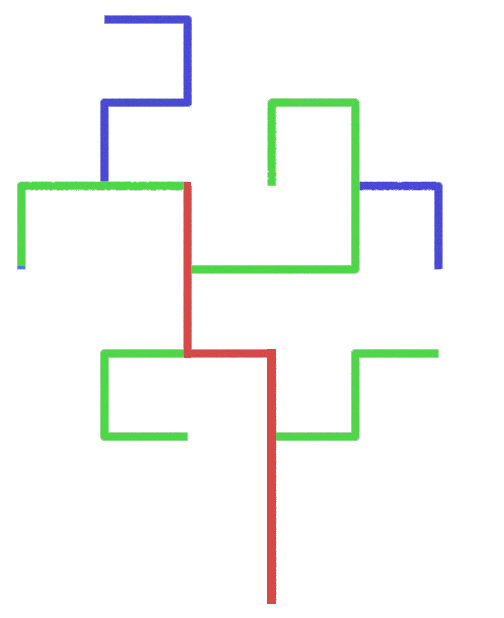
If turtle commands are placed inside square brackets [ ] the drawing point of the sequence jumps back to its position before the brackets. This way branches can be drawn from a main trunk
In the first example, only an initial premise string is used, consisting of F+- and [ ]
| Premise | FF[+F-F+F]F-F[F-F-F]+F[+FF-F[+F+F]F-F-F]F[-F[+F+F-F-F]F-F] |
| angle | 90 |
I have coloured the lines to show the main trunk, branches and nested branches. If I remove the branches is square brackets we are left with the simple instructions for the main trunk FFF-F+FF
Edge Rewrite
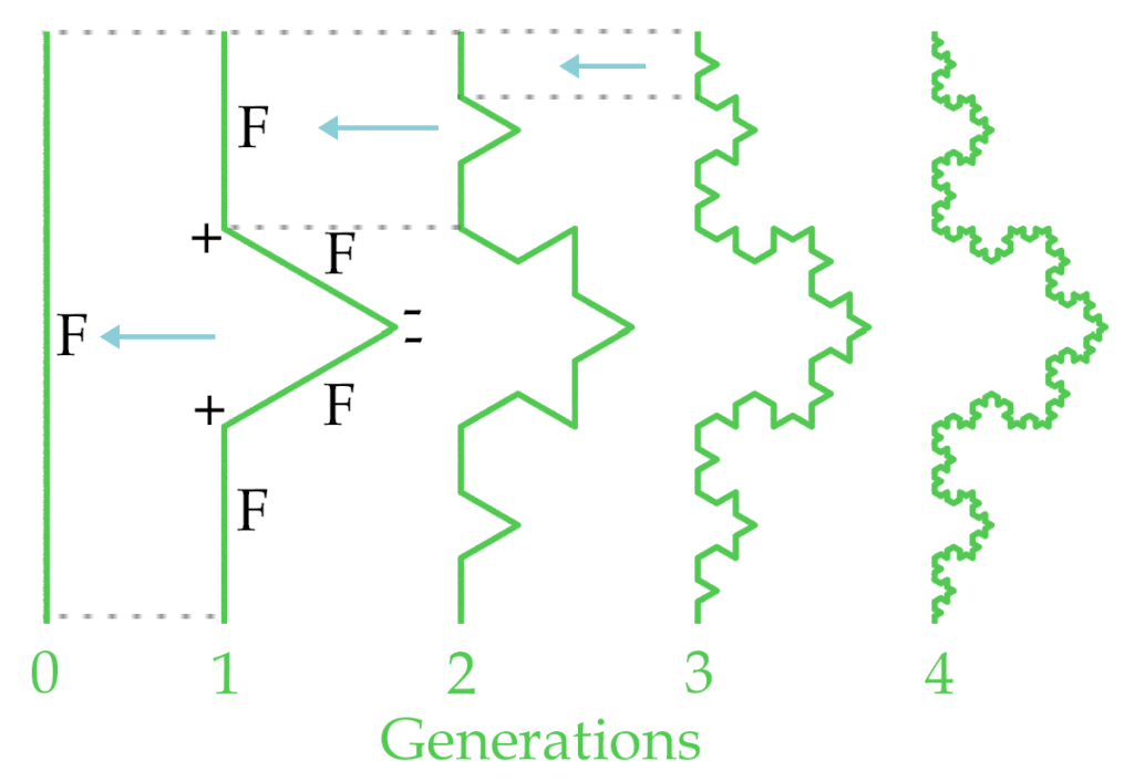
Each edge F is replaced by a new sequence. Here it is replaced by a line with a triangular detour which is drawn by the turtle sequence F+F–F+F
Every generation all the Fs are replaced again.
| Premise | F |
| Rule 1 | F=F+F–F+F |
| angle | 60 |
To keep the overall size constant divide the size of each new F by 3:
| Premise | F(1) |
| Rule 1 | F(i)=F(i/3)+F(i/3)–F(i/3)+F(i/3) |
| angle | 60 |
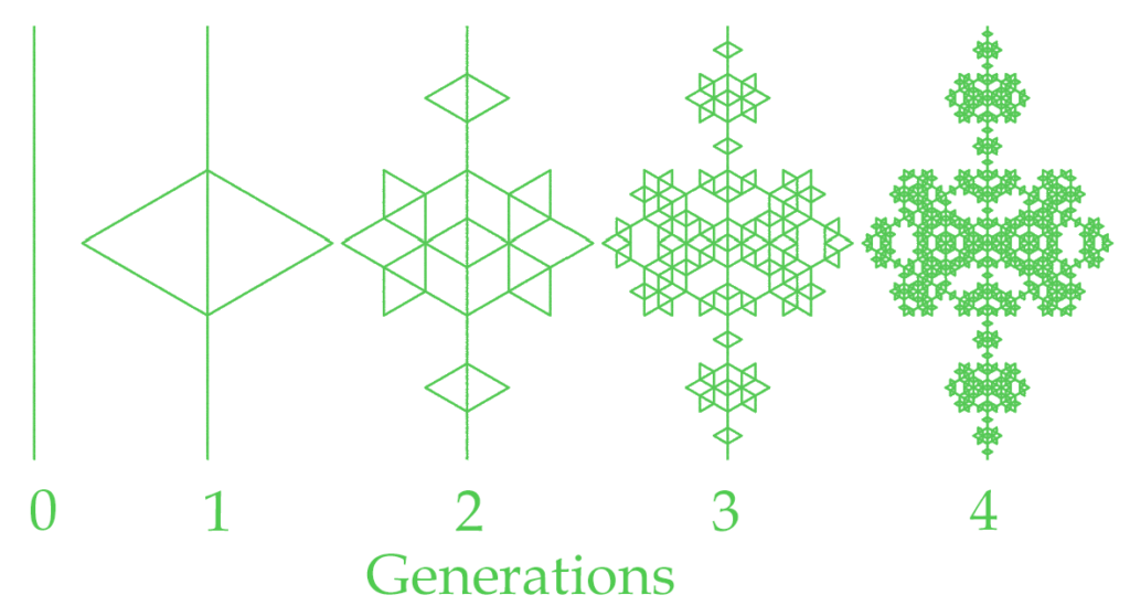
And here a different sequence FF++F++F+F++F-F inserts a diamond shape:
| Premise | F |
| Rule 1 | F=FF++F++F+F++F-F |
| angle | 60 |
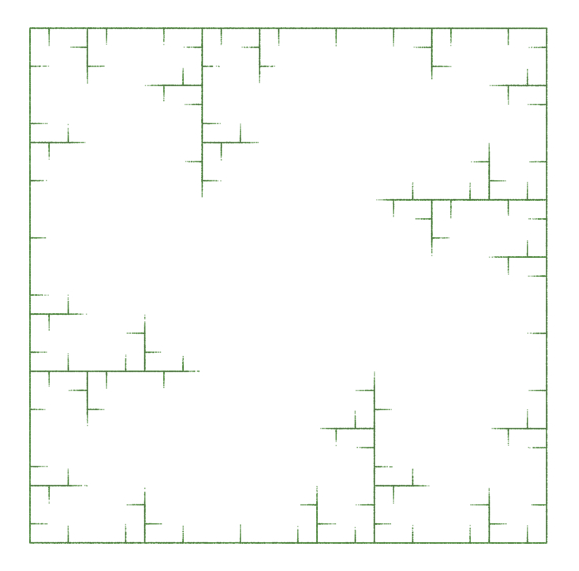
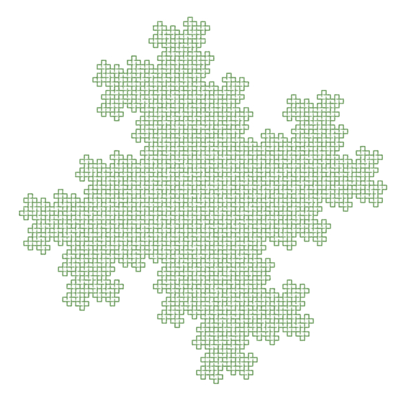
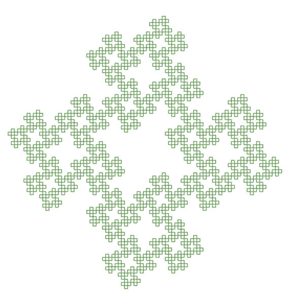
Edge Rewrite Examples from The Algorithmic Beauty of Plants p9 – p11.
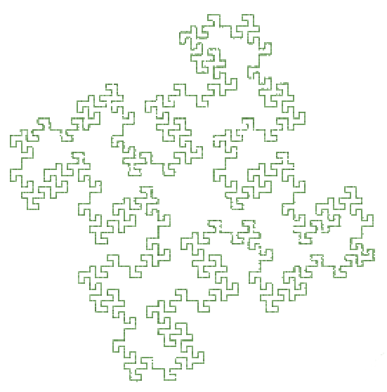 |  |  |  |
| Quadratic Koch Generations: 2 Premise: F-F-F-F Rule1: F=F+FF-FF-F- F+F+FF-F-F+F+FF+FF-F Angle:90 | Quadratic Snowflake Generations: 4 Premise: -F Rule1: F=F+F-F-F+F Angle:90 | Koch Curve a Generations: 4 Premise: F-F-F-F Rule1: F=FF-F-F-F-F-F+F Angle:90 | Koch Curve b Generations: 4 Premise: F-F-F-F Rule1:F=FF-F-F-F-FF Angle:90 |
 |  |  |  |
| Koch Curve c Generations: 3 Premise: F-F-F-F Rule1:F=FF-F+F-F-FF Angle:90 | Koch Curve d Generations: 3 Premise: F-F-F-F Rule1:F=FF-F–F-F Angle:90 | Koch Curve e Generations: 5 Premise: F-F-F-F Rule1:F=F-FF–F-F Angle:90 | Koch Curve f Generations: 5 Premise: F-F-F-F Rule1:F=F-F+F-F-F Angle:90 |
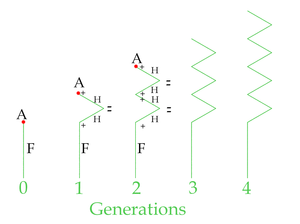
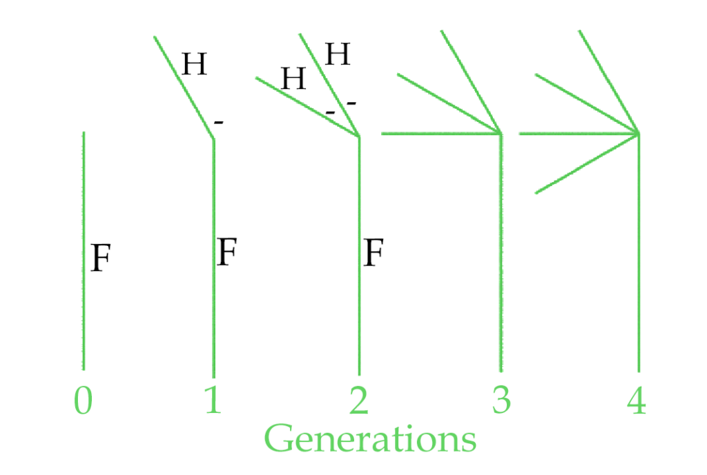
Node Rewrite
Instead of replacing an edge we can replace an unused character in our sequence with a new sequence. We can insert these characters anywhere. Commonly used characters are A, B, C, X as they are not otherwise used as Turtle commands.
In this example a node A is inserted at the end of the first F line (FA) In the second generation it is replaced with a triangular detour, and another A is added to the end (+H–H+A) and this is repeated to keep adding the same shape over and over again. Note H is a line half the size of F.
| Premise | FA |
| Rule 1 | A=+H–H+A |
| angle | 60 |
If the initial premise had been AFA the zigzag shapes would have been inserted at both the start and the end of the lines
In the second example a node A is inserted at the end of the first F line (FA). In the second generation A is inserted (to allow further iterations of the sequence) then the point turns 30 degrees, then a branch containing a half line is drawn, and the drawing point jumps back to just after the 30 degree turn.
| Premise | FA |
| Rule 1 | A=A-[H] |
| angle | 30 |
After each branch the angle (-) is added because it is outside the brackets, but the distance travelled by H is ignored.
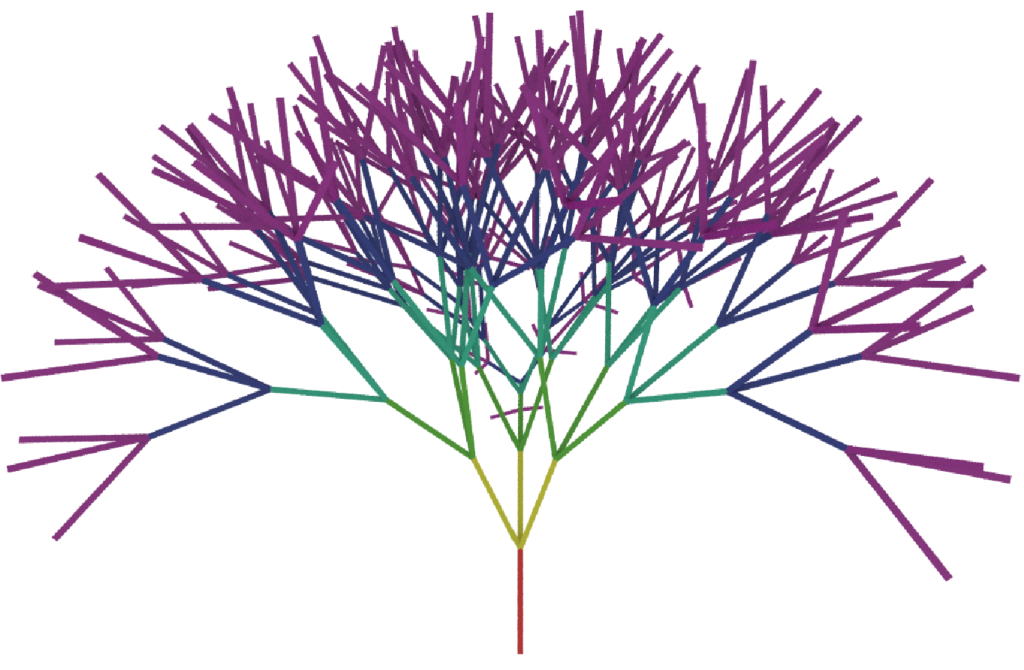
This example is a slightly simplified version of the Houdini default L-System settings. I have coloured each generation with a different colour to make it clearer how the tree grows.
This tree uses two rules, but it is pretty straightforward. Rule 1 establishes the branches. Rule 2 uses the B character to insert a rotated line at each branch.
| Premise | FFFA |
| Rule 1 | A=[B]////[B]////[B] |
| Rule 2 | B=&FFFA |
| angle | 28 |
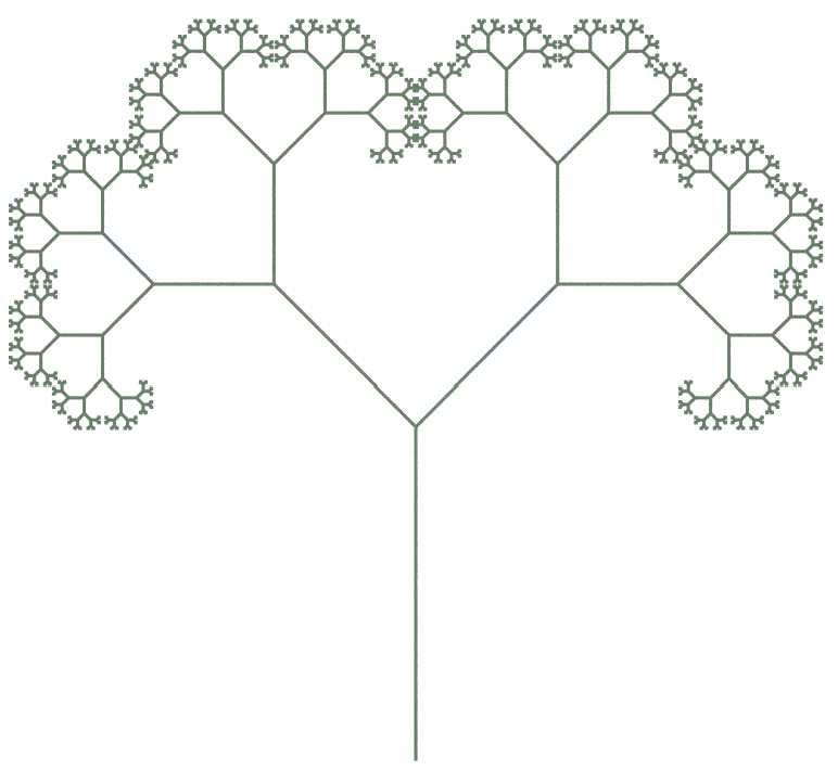
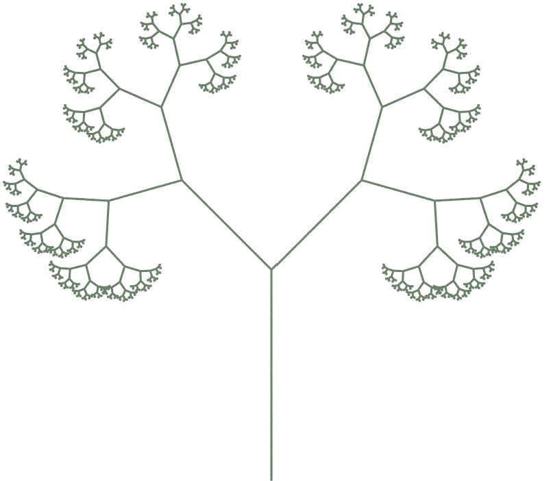
Branching Structures
from The Algorithmic Beauty of Plants p25. Also available as defaults ‘2D Plants’ in Houdini
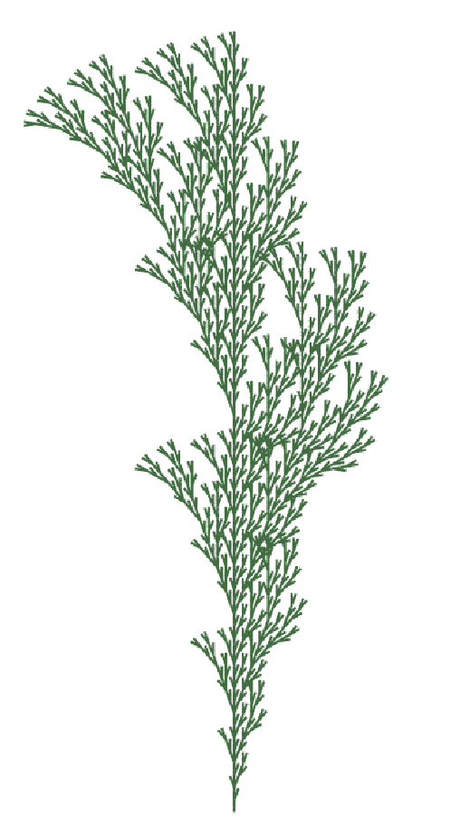
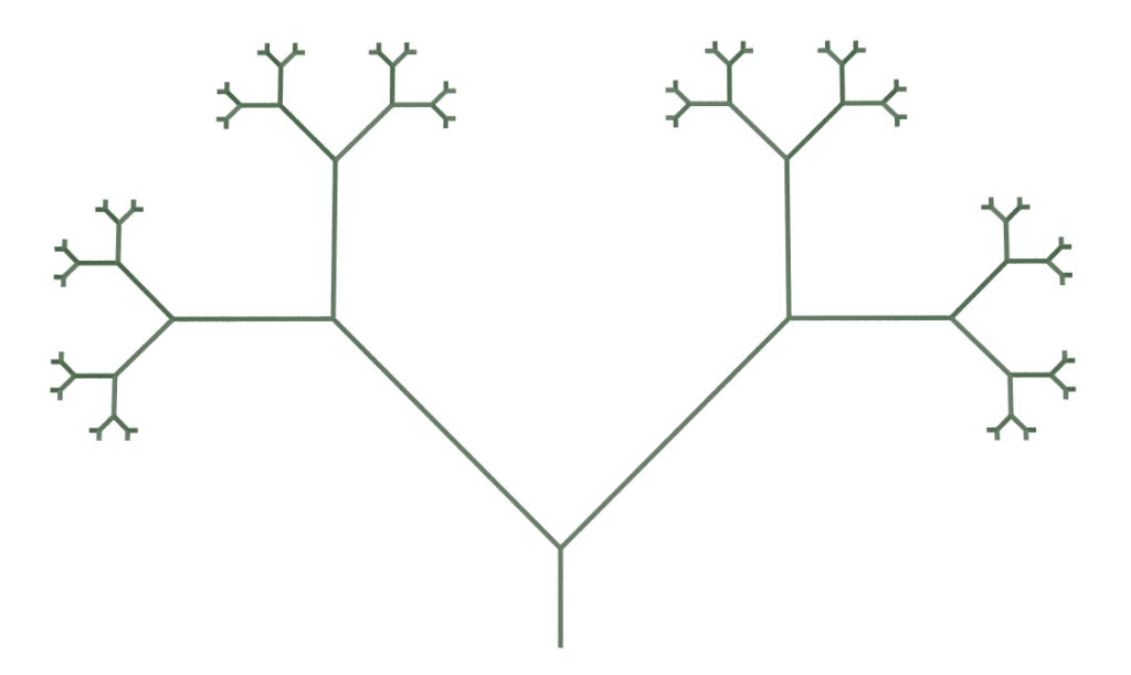
Figure 1.24: Examples of plant-like structures generated by bracketed OLsystems. L-systems (a), (b) and (c) are edge-rewriting, while (d), (e) and (f) are node-rewriting.
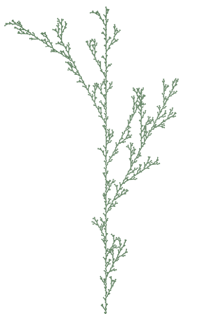 |  |  |
| a Generations: 4 Premise: F Rule1: F=F[+F]F[-F]F Angle:25 | b Generations: 5 Premise: F Rule1: F=F[+F]F[-F]F Angle:20 | c Generations: 4 Premise: F Rule1: F=F[+F]F[-F]F Angle:20 |
 |  |  |
| d Generations: 6 Premise: X Rule1: F=F[+F]F[-F]F Rule2:F=FF Angle:22.5 | e Generations: 6 Premise: X Rule1: X=F[+X][-X]FX Rule2:F=FF Angle:35 | f Generations: 6 Premise: X Rule1: X=F-[[X]+X]+F[+FX]-X Rule2:F=FF Angle:22.5 |
Symbol variables
You may have noticed that many of the turtle symbols have one or more optional variables after them. Usually they have a default value which can be edited in the ‘Values’ menu, or this can be inserted manually into the sequence and can be manipulated using simple maths. This gives us more control over the way the system changes over the generations.
| Symbols | Variables | Default Value if no Variable is specified | Variable Usage |
| F,f,H,h,G lines A, B, X etc. nodes to be replaced | (l,w,s,d) distance l of width w using s cross sections of d divisions each. | Stepsize | Usually you will just be working with the first (distance) and sometimes second (width) variables. Any unused variables to the right of these can be left out. |
| +,-,&,^,\,/,~ | (a) Angle in degrees | Angle | Use to override default angle |
| J,L,M geometry input | (s,x,a,b,c) Scale sx is unused a to c are stamping variables that can be used by the input geometry | Stepsize | Scale as a single variable can be used to override the default stepsize. If the stamping variables are needed, then scale must be set, followed by an empty or 0 value for x, then any stamping variables. |
| “, _ | (s) override step size scale | Step Size Scale. | Use to override default scale |
| !, ? | (s) override thickness scale | Thickness Scale(Tube menu) | Use to override default scale |
| ;, @ | (a) override angle scale | Angle Scale. | Use to override default scale |
Examples
 |  |  |  |  |
| Step Size = 0.2 Angle = 30 Premise: FA Rule1:A=A/[+FBJ] | Step Size = 0.2 Angle = 30 Premise: F(0.1)A Rule1:A=A/[+FBJ] | Step Size = 0.2 Angle = 60 Premise: FA Rule1:A=A/[+FBJ] | Step Size = 0.2 Angle = 60 Premise: FA Rule1: A=A/(30)[+FBJ] | Step Size = 0.2 Angle = 30 Premise: FA Rule1: A=A/[+FBJ(0.1)] |
| Uses Step Size & Angle from the values menu | The first F uses the given value of 0.1 | Changing the angle value changes both roll and turn (/ and +) | But setting the roll value in the rule keeps the spacing between branches constant, while still changing the Angle | Here we override the input sphere geometry size (J) so it no longer uses step size. (see “Input Geometry in L-Systems” below) |
Control variables over time
To set up a variable to change with each generation, you have to declare a value for it in the premise, then use a variable to represent this on both sides of the rule, and when a node or edge is declared for rewriting, manipulate this value (ie. add, multiply, divide a constant from it) This will be iterated every time the edge or node is replaced.
The effect achieved is similar to using the scale values “, _,!, ?,;, @ but with greater control
From the L-System documentation:
To create an L-system which goes forward x percent less on each iteration, you need to start your Premise with a value, and then in a rule multiply that value by the percentage you want to remain.
Premise A(1)
Rule A(i)= F(i)A(i*0.5)
This way i is scaled before A is re-evaluated. The important part is the premise: you need to start with a value to be able to scale it.
Usage in a branching tree:
This example uses a simplified 2D version of the default branching L-System
| Premise | FFFA(1) |
| Rule 1 | A(i)=[&F(i)A(i*0.5)]////[&F(i)A(i*0.5)] |
| angle | 45 |
| generations | 6 |
Every time A is declared in rule 1, the value i (length) is halved so each generation starts with a smaller value.
Using Custom Values
In order to make an L-System easier to edit you can replace the variables in your rules with custom values from the ‘Values’ menu. By default there are three of these, b, c and d, but there are options to add as many more of them as you want, and supply your own letters for them. This can make it much easier to tweak the settings of your L-System. It is a technique that is extensively used in The Algorithmic Beauty of Plants for their trees. These trees are available in the Houdini presets menu, but in my examples I have added an extra menu to tweak the values more easily.
Monopodial Tree
The Algorithmic Beauty of Plants p.56, figure 2.6, also shown by the Houdini preset “Monopodial Tree”
| Premise | A(1,10) |
| Rule 1 | A(l,w)=F(l,w)[&(c)B(l*e,w*h)]/(m)A(l*b,w*h) |
| Rule 2 | B(l,w)=F(l,w)[-(d)$C(l*e,w*h)]C(l*b,w*h) |
| Rule 3 | C(l,w)=F(l,w)[+(d)$B(l*e,w*h)]B(l*b,w*h) |
Custom Values
b = contraction ratio trunk
e = contraction ratio branches
c = branching angle trunk
d = branching angle lateral axes
h = width decrease rate
i = divergence angle
For each tree below the rules are the same, only the values are changed.
 |  |  |  |
| b = 0.9 e = 0.6 c = 45 d = 45 h = 0.707 i = 137.5 | b = 0.9 e = 0.9 c = 45 d = 50.6 h = 0.707 i = 137.5 | b = 0.9 e = 0.8 c = 45 d = 45 h = 0.707 i = 137.5 | b = 0.9 e = 0.7 c = 30 d = -30 h = 0.707 i = 137.5 |
Sympodial Tree
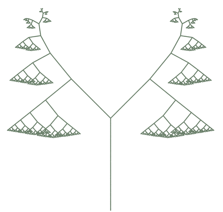
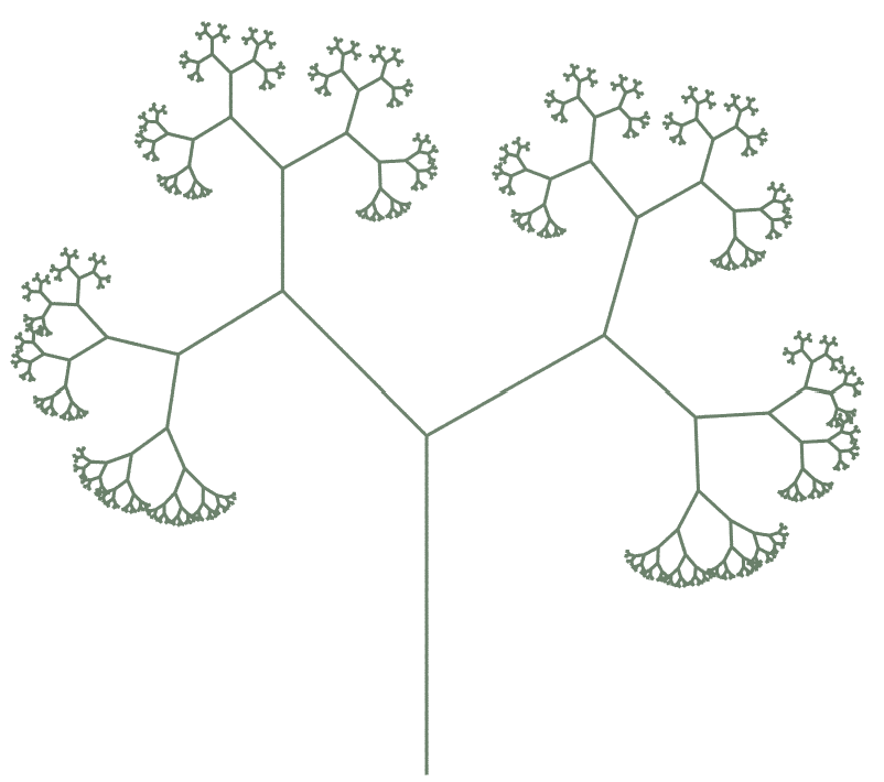
The Algorithmic Beauty of Plants p.59, figure 2.7, also shown by the Houdini preset “Sympodial Tree”
| Premise | A(1,10) |
| Rule 1 | A(l,w)=F(l,w)[&(c)B(l*b,w*h)]//(180)[&(d)B(l*e,w*h) |
| Rule 2 | B(l,w)=F(l,w)[+(c)$B(l*b,w*h)][-(d)$B(l*e,w*h)] |
Custom Values
b = contraction ratio 1
e = contraction ratio 2
c = branching angle 1
d = branching angle 2
h = width decrease rate
For each tree below the rules are the same, only the values are changed.
 |  |  |  |
| b = 0.9 e = 0.7 c = 5 d = 65 h = 0.707 | b = 0.9 e = 0.7 c =10 d = 60 h = 0.707 | b = 0.9 e = 0.8 c = 20 d = 50 h = 0.707 | b = 0.9 e = 0.8 c = 35 d = 35 h = 0.707 |
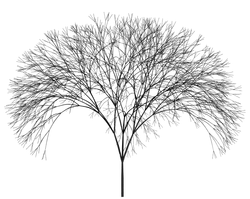
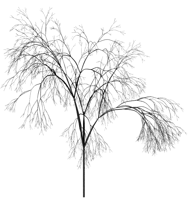
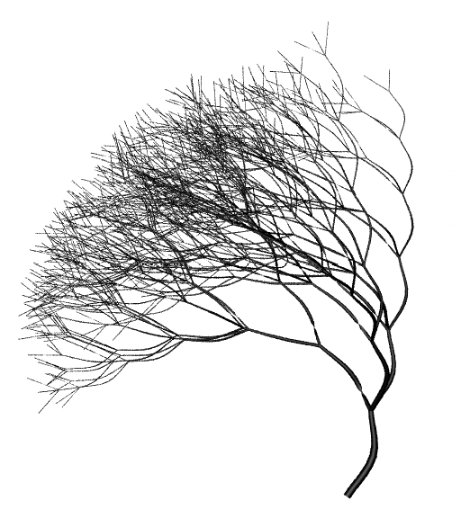
Gravity (tropism)
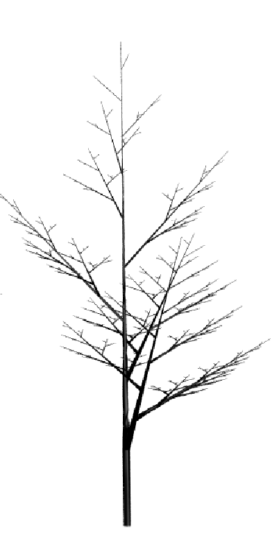
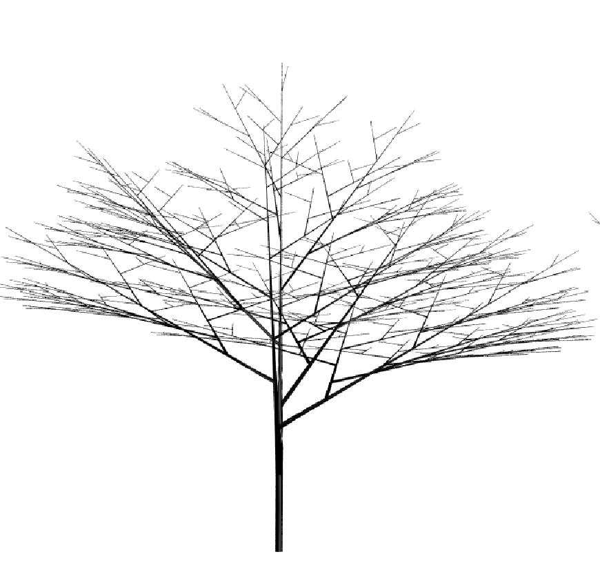
Adding the variable T to an L-System adds gravity in the -Y direction. This will increase over the generations if it is called with each generation. It can also be inserted into a branch so it only effects that branch
 |  |
| Premise= FA Rule 1= A=T“[&FA]////[&FA] Angle= 45 Step Size Scale= 0.6 Generations= 10 Gravity= 0 | Premise= FA Rule 1= A=T“[&FA]////[&FA] Angle= 45 Step Size Scale= 0.6 Generations= 10 Gravity= 20 |
 |  |
| Premise= FA Rule 1= A=T“[&FA]////[&FA] Angle= 45 Step Size Scale= 0.6 Generations= 10 Gravity= 50 | Premise= FA Rule 1= A=”[&TFA]////[&FA] Angle= 45 Step Size Scale= 0.6 Generations= 10 Gravity= 20 |
Ternary Tree
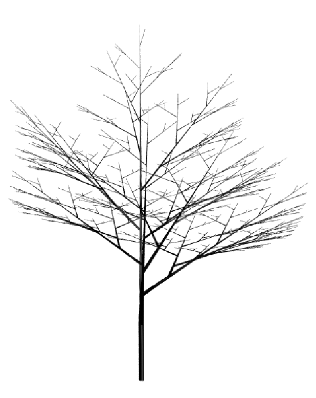
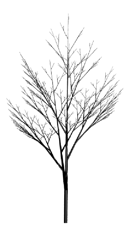
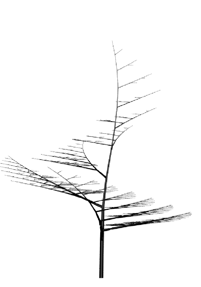
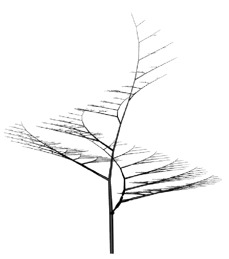
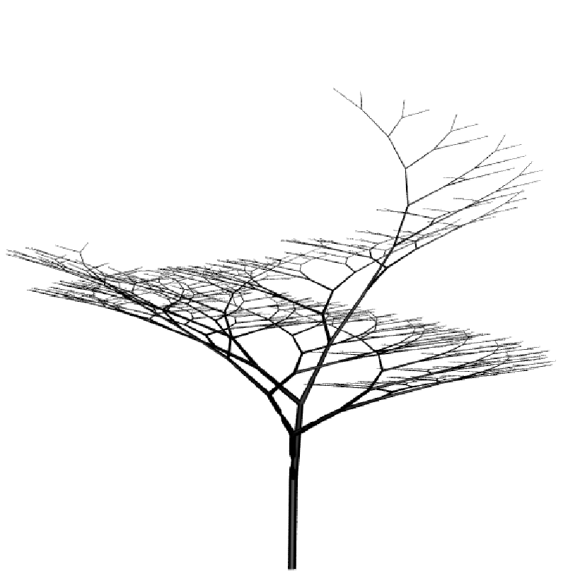
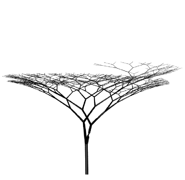
The Algorithmic Beauty of Plants p.60, figure 2.8, also shown by the Houdini preset “Ternary Tree”
| Premise | F(0.5,1)A |
| Rule 1 | A=TF(0.5,1)[&(c)F(0.5,1)A]/(b)[&(c)F(0.5,1)A]/(e)[&(c)F(0.5,1)A] |
| Rule 2 | F(l,w)=F(l*d,w*h) |
Custom Values
b = divergence angle 1
e = divergence angle 2
c = branching angle
d = elongation rate
h = width increase rate
T = tropism (gravity)
For each tree below the rules are the same, only the values are changed. The exception is the final tree which is grown at an angle using the initial premise +(75)F(0.5,1)A. This allows T to pull the tree to one side instead of directly downwards. It is then rotated back into an upright position using a transform node.
 |  |  |  |
| b = 94.64 e = 132.63 c = 18.95 d = 1.109 h = 1.732 T = 15 | b =137.5 e = 137.5 c =18.95 d = 1.109 h = 1.452 T = 12 | b = 112.5 e = 157.5 c = 22.5 d = 1.356 h = 1.653 T = 21 | b = 180 e = 252 c = 36 d =1.07 h =1.529 T = 27.5 Premise = +(75)F(0.5,1)A |
Input Geometry in L-Systems
The L-System node has three geometry inputs which allow you to hook up any piece of geometry and use it in your L-System. J, K and M respectively. Any geometry connected to these inputs is created in the sequence by these letters
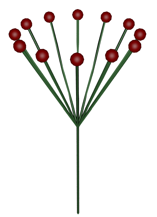
This example uses the default L-System tree again.
It adds leaf geometry [&&J] before each occurance of [B]. The brackets are used so that the pitch (&&) rotates the leaves but doesn’t affect the rest of the system. It also adds a berry geometry K at the end of each branch.
| Premise | FFFA |
| Rule 1 | A=!”[&&J][B]////[&&J][B]////[&&J]B |
| Rule 2 | B=&FFFAK |
| angle | 28 |
A plant generated by an L-system, The Algorithmic Beauty of Plants p.27, Figure 1.26
 |  |
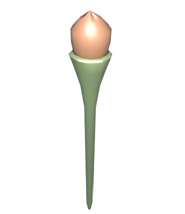
| J | K |
| Premise | A |
| Rule 1 | A=X+[A+]−−////[−−J]X[++J]−[A]++AK |
| Rule 2 | X=FY[//&&J]FY |
| Rule 3 | Y=YFY |
| angle | 18 |
| Generations | 5 |
Stamping Geometry
You can use the stamp expression to influence the inputs to an L-System. The syntax to use is
stamp(“/path/to/lsystem”, “lsys”,0)
The “lsys” variable can be changed inside the l-system using the parameters after the J, K or M symbols
| J(s,x,a,b,c) etc | The geometry is scaled by the s parameter (default Step Size) and stamped with the values a through c (default no stamping). Stamping occurs if the given parameter is present and the relevant Leaf parameter is set. The x parameter is not used and should be set to 0. |
So to change the parameters of the stamped input use eg.
J(0.1, 0, ”value for stamping”)
Note that the documentation suggests the following will work J(,,”value for stamping”) but in practice this doesn’t create any geometry, which seems to be a bug.
Example using stamp expression to choose geometry
Input Geometry connected to inputs 0 to 3 of a switch node:
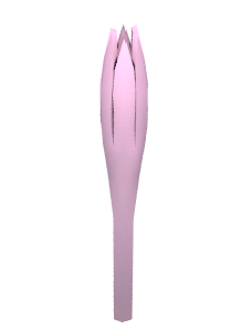 |  |  |  |
The switch node is connected to input J of an L-System set up as shown below. The ‘Select ‘Input’ parameter of the switch node has the expression
stamp(“../lsystem1″,”lsys”,0)
The sequence here is very straightforward. For every generation a straight line F is drawn upwards and 3 nodes B are branched off around the trunk.
These nodes are then replaced with the input connected to J
The stamping selects which input of the switch node connected to J is used. To determine the value connected to the third variable in J we use the ‘t’ character which returns the number of iterations. This starts at 1 at the top and descends to the last generation (21) at the bottom. We divide t by a variable b of about 4.5 to give us a number between 1 and 4 (representing the 4 inputs) then subtract 1 to give us 0 to 3. Changing the value of b in the values menu changes the positions at which the leaf/flower types change.
| Premise | FA |
| Rule 1 | A=AF//[+&B]//[&B]//[&B] |
| Rule 2 | B=J(1, 0, t/b-1) |
| Step size | 0.45 |
| angle | 48 |
| Variable b | 4.5 (try changing this) |
| Generations | 21 |

Example using stamp expression to change colour
In this example we only have one geometry model, and we use stamping to change the colour.
| The input flower has a colour node with the following expressions for RGB:R: 0.5+stamp("../lsystem1","lsys",0)/20 |
The l-system is very similar to above, except that the J third character value is simply ‘t’ which is tweaked in the colour node to give an output between 0 and 1, and the first (scaling) character of J also uses ‘t’ to make the petals smaller as they ascend.
| Premise | FA |
| Rule 1 | A=A”!F//[+&B] |
| Rule 2 | B=J(0.5+t/10,0,t) |
| Step size | 0.65 |
| angle | 48 |
| Generations | 21 |

Probability
Appending a colon followed by a fraction to the end of a rule determines how often that rule is applied
Eg. B=&FFFAK:0.75
would replace B with &FFFAK only ¾ of the time. This is a good way to introduce more natural looking dropoup to L-Systems.
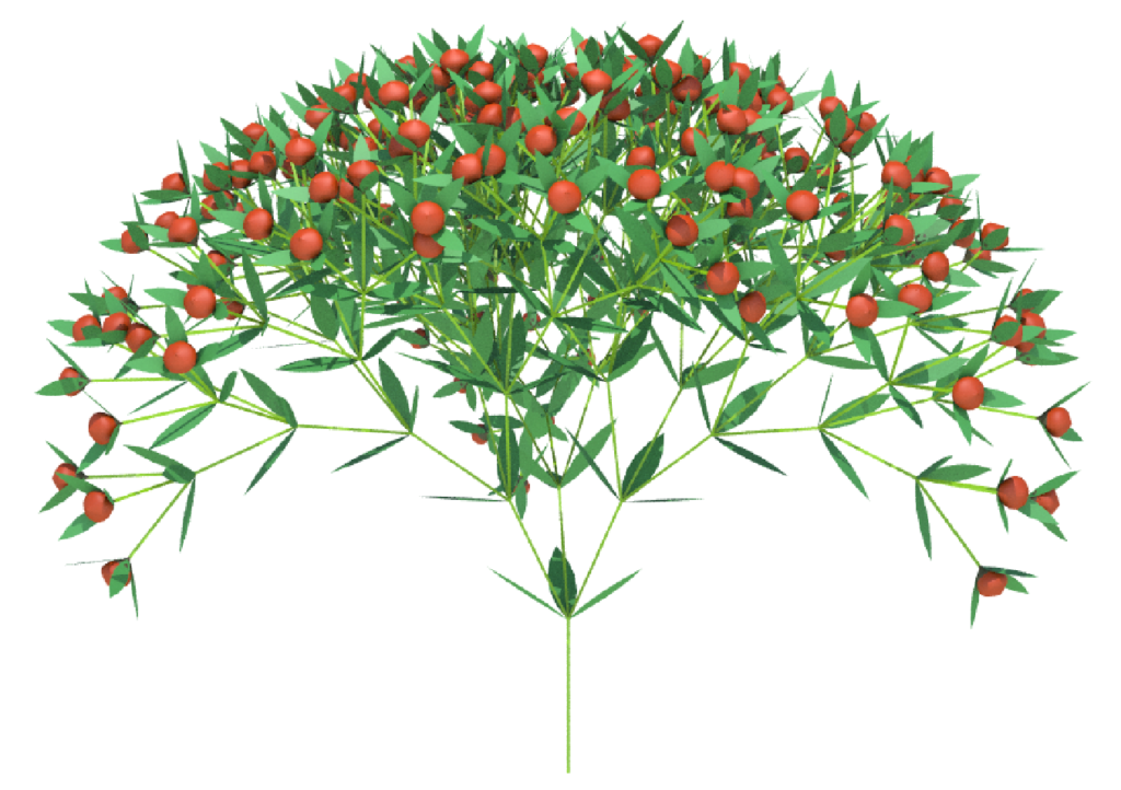
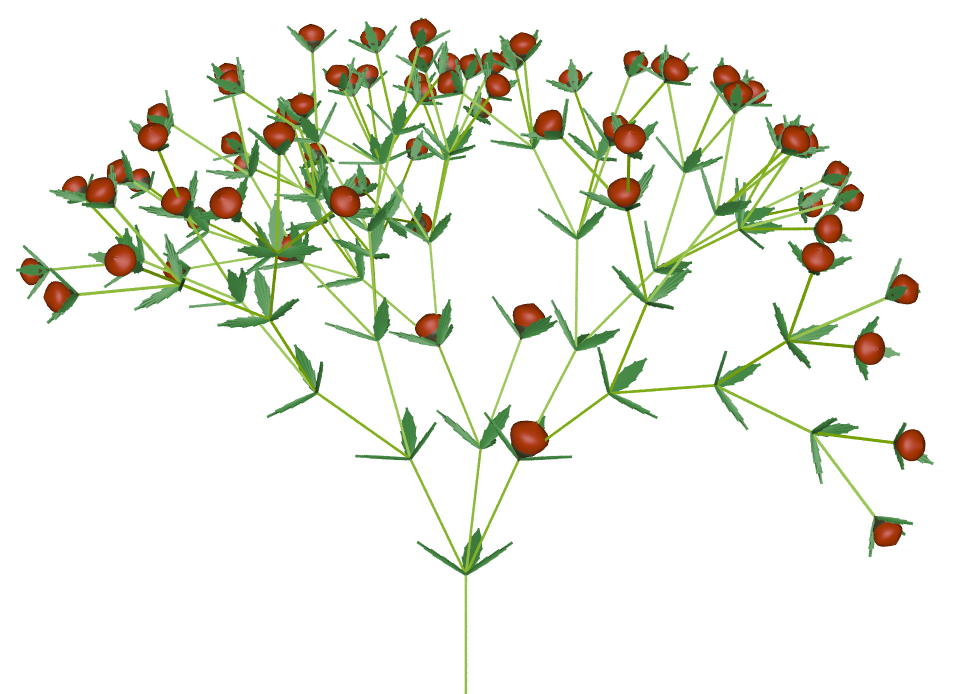
This example is a copy of the default L-System with geometry leaves and berries, only this time the second rule only executes in 75% of cases (:0.75)
This gives a much more natural appearance. Note that more than 25% of the foliage is missing because some branches drop out earlier on eliminating everything above them.
| Premise | FFFA |
| Rule 1 | A=!”[&&J][B]////[&&J][B]////[&&J]B |
| Rule 2 | B=&FFFAK:0.75 |
| angle | 28 |
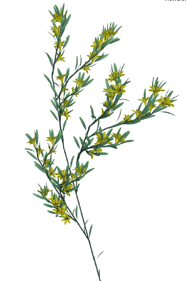
In this version a second Rule is added containing flower geometry and both rules are given low probability
| Rule 2 | B=&FFFAK:0.45 |
| Rule 3 | B=&FFFAM:0.25 |
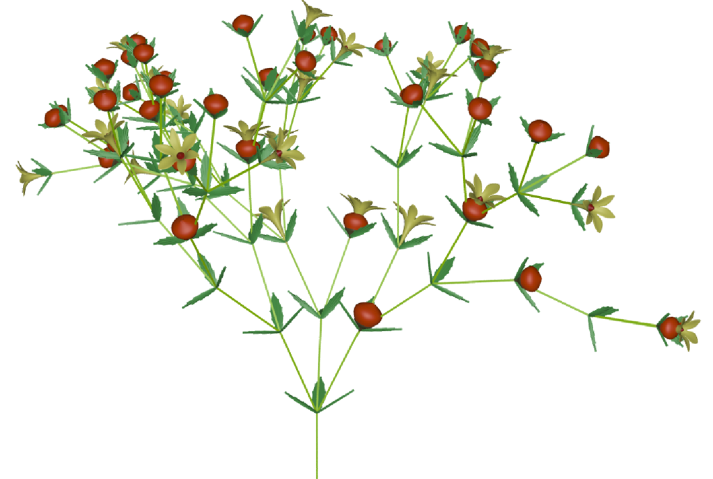
Changing ‘seed’ in the geometry menu will give a different random dropout
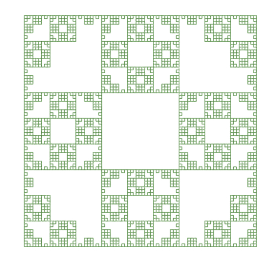
Example of probability from The Algorithmic Beauty of Plants p.28
Stochastic L-systems
| Premise | F |
| Rule 1 | F=F[-F]F[+F]F:0.33 |
| Rule 2 | F=F[-F]F:0.33 |
| Rule 3 | F=F[+F]F:0.33 |
| angle | 28 |
| Generations | 6 |

Conditionals
We can add a condition to an L_Systems rule so that it only executes when the condition is true. The symbol for a conditional is a colon : after which the condition is given. For example
A:t<4=J
This would replace A with geometry input J only for the first 4 iterations
In this example there is a single leaf geometry input (J)  There are two rules. The first is used for the first iteration. It places a single leaf at the end of a short branch. The second rule is used for all other iterations (ie. generations). It places two leaves angled away from the main branch.
Increasing the generations always adds more pairs of leaves
| Premise | A |
| Rule 1 | A:t>1=AF[+J][-J] |
| Rule 2 | A:t==1=AH[J] |
| angle | 60 |


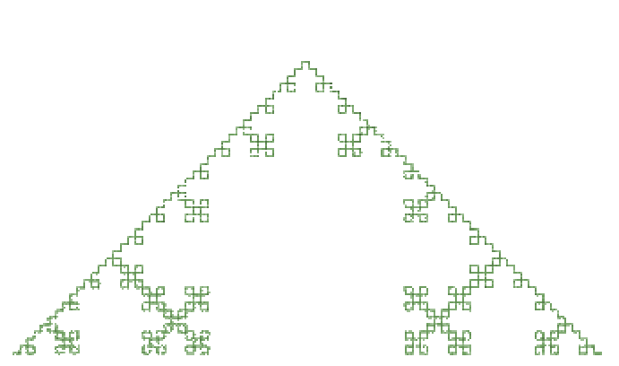
Conditional Edge Rewrite Examples from The Algorithmic Beauty of Plants p9 – p11.
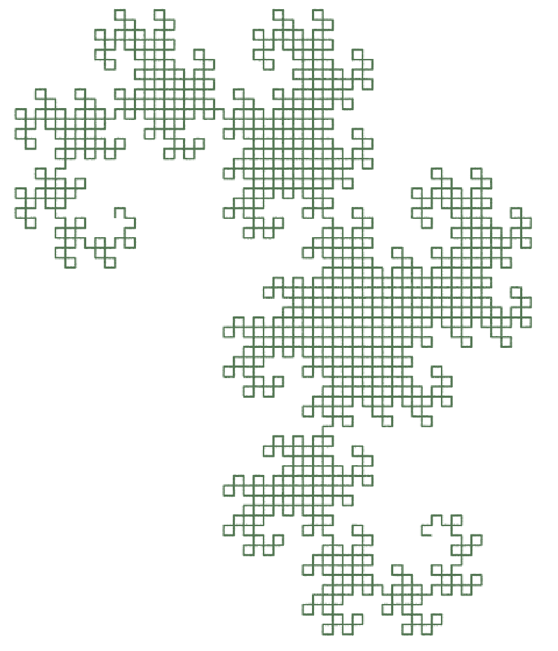 | 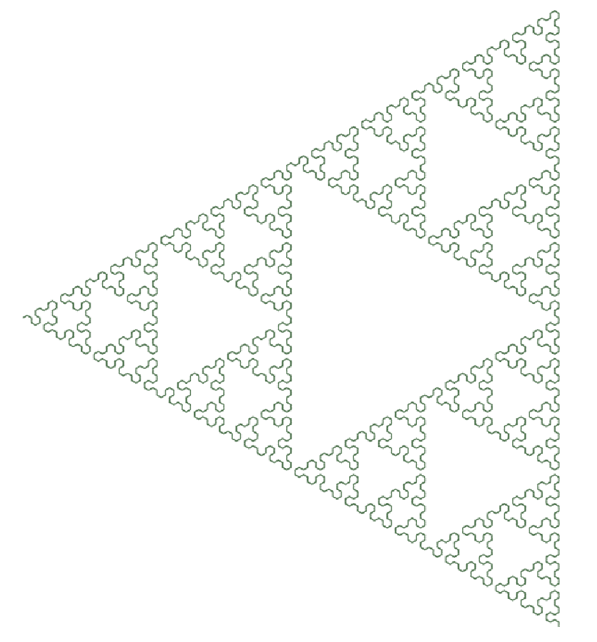 |
| Dragon_curve Generations: 12 Premise: l Rule1: l:t<b=l+r+ Rule2: r:t<b=-l-rRule1: l=F Rule1: r=F Angle:90 Variable b: ch(“generations”) (ie. 12) | Sierpinski_gasket Generations: 8 Premise: r Rule1: l:t<b=r+l+r Rule2: r:t<b=l-r-l Rule1: l=F Rule1: r=F Angle:60 Variable b: ch(“generations”) (ie. 8) |
Bringing together Geometry Inputs, Custom Variables and Conditionals
 J(,,0)
  J(,,1)
  K(,,0)
 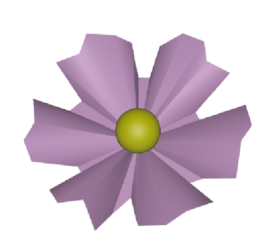 K(,,1)
 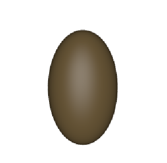 K(,,2)
| Premise | A(7) |
| Rule 1 | A(i):i==7=FI(20)[&(60)∼J(0)]/(90)[&(45)A(0)]/(90)[&(60)∼J(0)]/(90)[&(45)A(4)]FI(10)∼K(0,0,0) |
| Rule 2 | A(i):i<7=A(i+1) |
| Rule 3 | I(i):i>0=FFI(i-1) |
| Rule 4 | J(i)=J(i+1,0,(i+1)/t) |
| Rule 5 | K(i)=K(i+1,0,(i+1)/15) |
| Generations | 40 |
Context Sensitive L-Systems
From The Algorithmic Beauty of Plants p.30
A context-sensitive extension of tree L-systems requires neighbor Context in tree edges of the replaced edge to be tested for context matching. 2L-systems use productions of the form a <b>c → χ where the letter b (called the strict predecessor) can produce word χ if and only if b is preceded by letter a and followed by c.
This can be used in Houdini if the option “Context includes Siblings” is turned on.
Note that the > and < signs don’t mean “greater than” or “less than”, they mean “comes after” or “comes before”.
Example of Context sensitive leaf drawing
In this example, there are two conditions for drawing leaf geometry (J)
- If B comes after A and before A, a leaf is drawn to the left
- If A comes after B and before A, a leaf is drawn to the right
| Premise | BABAABBA |
| Rule 1 | A<B<A=[—J] B |
| Rule 2 | B<A<B=[+++J] A |
| Rule 3 | A=-F |
| Rule 4 | B=+F |
| angle | 20 |
| Generations | 5 |
The result of these rules is that leaves are only drawn when the direction changes and are always situated on outside curves.

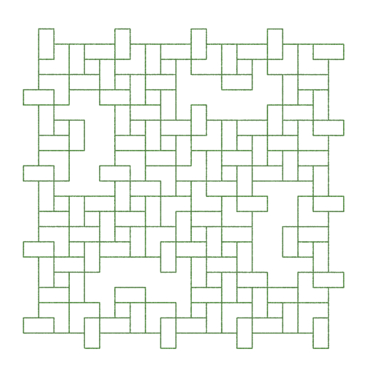
Examples of branching structures generated using L-systems based on the results of Hogeweg and Hesper. The Algorithmic Beauty of Plants p.34
 |  |  |  |  |
| Generations: 25 Premise: FBFBFB Rules: A<A>A = A A<A>B = B[+FBFB] A<B>A = B A<B>B = B B<A>A = A B<A>B = BFB B<B>A = A B<B>B = A + = – – = + Angle:22.5 | Generations: 30 Premise:FBFBFB Rules: A<A>A = B A<A>B = B[-FBFB] A<B>A = B A<B>B = B B<A>A = A B<A>B = BFB B<B>A = B B<B>B = A + = – – = + Angle:22.5 | Generations: 26 Premise:FBFBFB Rules: A<A>A = A A<A>B = B A<B>A = A A<B>B = B[+FBFB] B<A>A = A B<A>B = BFB B<B>A = A B<B>B = A + = – – = + Angle:25.75 | Generations: 26 Premise:FAFBFB Rules: A<A>A = B A<A>B = A A<B>A = A A<B>B = BFB B<A>A = B B<A>B = B[+FBFB] B<B>A = B B<B>B = A + = – – = + Angle:25.75 | Generations: 26 Premise:FAFAFA Rules: B<B>B = B B<B>A = A[-FAFA] B<A>B = A B<A>A = A A<B>B = B A<B>A = AFA A<A>B = A A<A>A = B + = – – = + Angle:22.5 |
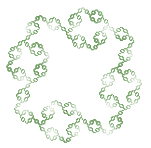
Phyllotaxis
Phyllotaxis refs to the arrangement of petals or seeds in a flower head. The key to this is the Fibonacci angle, approximately equal to 137.5◦. The angle is the result of dividing a circle by the golden ratio.
The central illustration below gives the basic L-System rule used to create the pattern. The patterns to the left and right demonstrate how much the pattern changes when the angle is changed by a fraction of a degree.
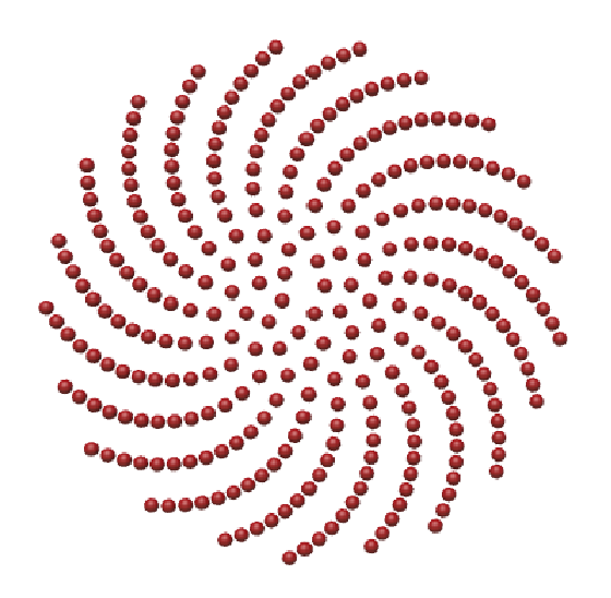 | 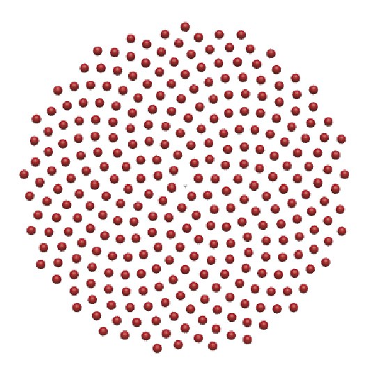 | 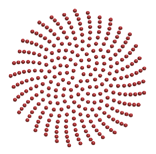 |
| Premise: A(1) Rule 1: A(n) = +(137.3)[f(n^0.5)J]A(n+1) Step Size: 1 Generations: 300 | Premise: A(1) Rule 1: A(n) = +(137.5)[f(n^0.5)J]A(n+1) Step Size: 1 Generations: 300 | Premise: A(1) Rule 1: A(n) = +(137.6)[f(n^0.5)J]A(n+1) Step Size: 1 Generations: 300 |
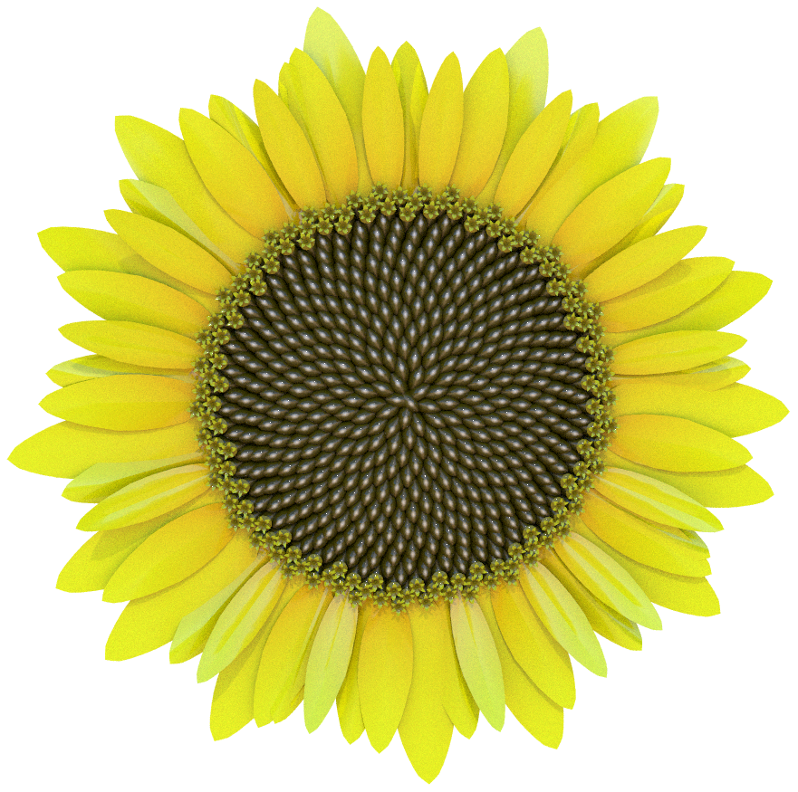
Sunflower
The sunflower uses a single rule to draw the seeds and petals. The only change is that the seeds become petals as the generations increase, which is done using Conditionals
 J
J  K
K 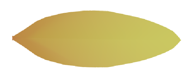 M(,,0)
  M(,,1)
  M(,,2)
  M(,,3)
| Premise | A(0) |
| Rule 1 | A(n) = +(137.5)[“f(n^0.5)C(n)]A(n+1) |
| Rule 2 | C(n) : n <= 440 = J |
| Rule 3 | C(n) : 440 < n & n <= 565 = K |
| Rule 4 | C(n) : 565 < n & n <= 580 = M(1,0,0) |
| C(n) : 580 < n & n <= 595 = M(1,0,1) | |
| C(n) : 595 < n & n <= 610 = M(1,0,2) | |
| C(n) : 610 < n = M(1,0,3) | |
| Step Size | 1 |
| Generations | 625 |
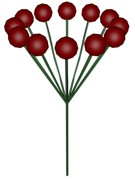
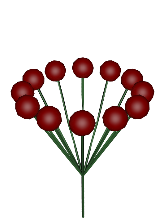
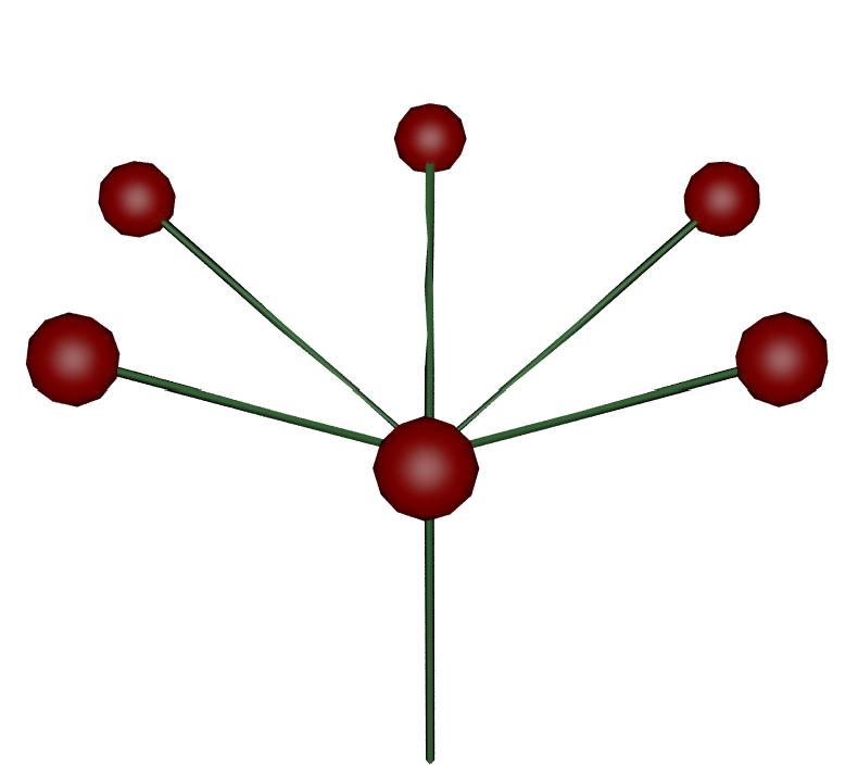
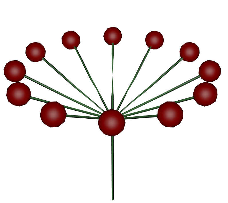
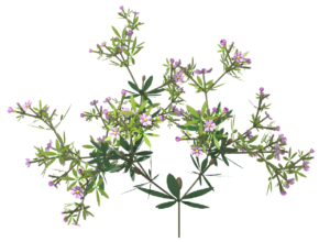
The same principle can be used to create flowerheads. In this flower the angle and size of the petals is increased as they get further from the centre (as n becomes greater)
The & symbol in rule 2 is used to rotate the petals outwards as the generations increase. Variable b is linked to the total number of generations. This is also used to grow the petals as they get further out.
| Premise | A(0) |
| Rule 1 | A(n) = +(137.5)[“f(n^0.5)C(n)]A(n+1) |
| Rule 2 | C(n)=&(n*-180/b)J(0.5+(b-n)/b) |
| Step Size | 1 |
| Variable b | ch(“generations”) |
| Generations | 90 |

Creating Leaves from Surface Geometry
It is possible to use L-Systems to draw polygon surfaces, using the following commands:
{ Start a polygon
. Make a polygon vertex
} End a polygon
The Algorithmic Beauty of Plants contains several examples of surfaces built from polygons, and one of these is integrated into the houdini L-System examples as ‘Cordate Leaf’
Cordate Leaf
The Algorithmic Beauty of Plants p.123, Figure 5.5
This is created by drawing polygon triangles and joining them up to form the shape of a leaf. If we look at the turtle generated for each generation we can see that the rules add progressively longer lines (lists of FFF), and join these up with progressively wider angles (lists of +++)
| Premise | [A][B] |
| Rule 1 | A=[+A{.].C.} |
| Rule 2 | B=[-B{.].C.} |
| Rule 3 | C=FFFC |
| Angle | 16 |
The results below show only the right side for simplicity ie. they ignore rule 2
Gen 0 [A]
Gen 1 [[+A{.].C.}]
Gen 2 [[+[+A{.].C.}{.].FFFC.}]
Gen 3 [[+[+[+A{.].C.}{.].FFFC.}{.].FFFFFFC.}]
Gen4 [[+[+[+[+A{.].C.}{.].FFFC.}{.].FFFFFFC.}{.].FFFFFFFFFC.}]
 |  |  |  |
| 3 Generations | 4 Generations | 6 Generations | 12 Generations |
A family of simple leaves
The Algorithmic Beauty of Plants p.124, Figure 5.6
| Premise | {.A(0)} |
| Rule 1 | A(i) = F(b,c)[-B(i).][A(i+1)][+B(i).] |
| Rule 2 | B(i):i>0 = F(d,e)B(i-f) |
| Rule 3 | F(s,r) = F(s*r,r) |
| Angle | 60 |
| generations | 20 |
Variable Values Represent:
b = initial length – main segment
c = growth rate – main segment
d = initial length – lateral segment
e = growth rate – lateral segment
f = growth potential decrement
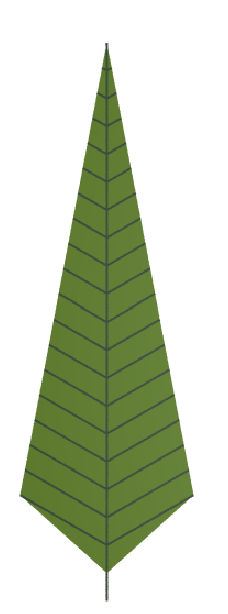 | 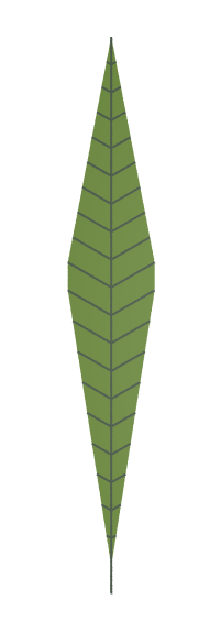 | 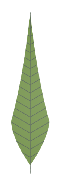 | 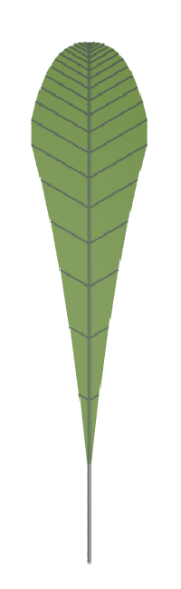 | 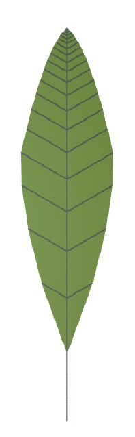 | 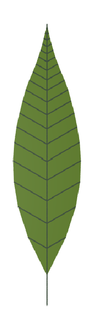 |
| b = 5 c = 1 d = 1 e = 1 f = 0 | b = 5 c = 1 d = 1 e = 1 f = 1 | b = 5 c = 1 d = 0.6 e = 1.06 f = 0.25 | b = 5 c = 1.2 d = 10 e = 1 f = 0.5 | b = 5 c = 1.2 d = 4 e = 1.1 f = 0.25 | b = 5 c = 1.1 d = 1 e = 1.2 f = 1 |
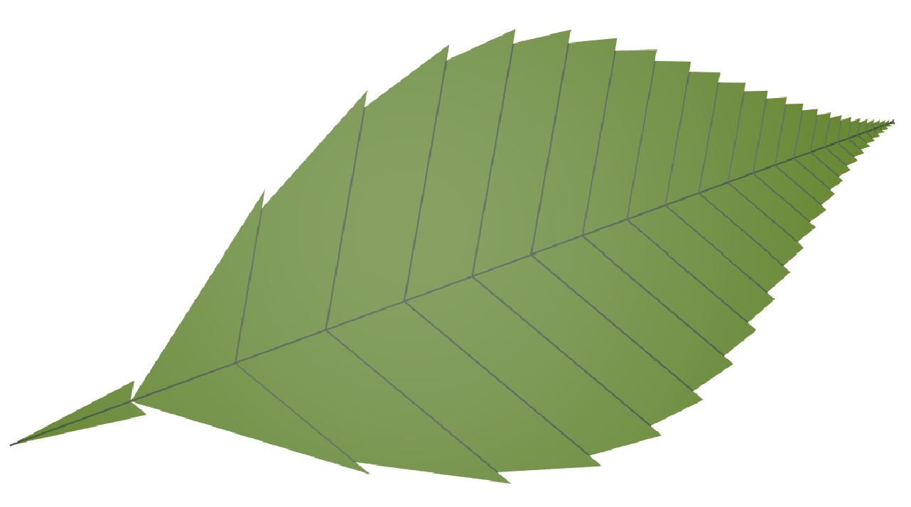
A Rose Leaf
From The Algorithmic Beauty of Plants p.126, Figure 5.8
| Premise | [{A(0).}][{C(0).}] |
| Rule 1 | A(i) = .F(b,c).[+B(i)F(f,h,i).}][+B(i){.]A(i+1) |
| Rule 2 | C(i) = .F(b,c).[-B(i)F(f,h,i).}][-B(i){.]C(i+1) |
| Rule 3 | B(i) : i>0 = F(d,e)B(i-1) |
| Rule 4 | F(s,r)=F(s*r,r) |
| Rule 5 | F(s,r,i) : i>1 = F(s*r,r,i-1) |
| Angle | 60 |
| generations | 25 |
 Variable Values Represent:
b = 5 : initial length – main segment
c = 1.15 : growth rate – main segment
d = 1.3 : initial length – lateral segment
e = 1.25 : growth rate – lateral segment
f = 3 : initial length – marginal notch
h = 1.09 : growth rate – marginal notch
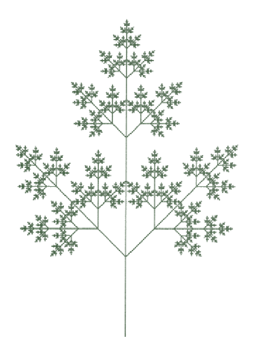
Ferns and other Compound Leaves
From The Algorithmic Beauty of Plants p.129, Figure 5.11
- b = apical delay (number of children on a frond, a whole number)
- c = internode elongation rate (decrease in size of fronds)
| Premise | A(0) |
| Rule 1 | A(i):i>0 = A(i-1) |
| Rule 2 | A(i):i==0 = F(1)[+A(b)][-A(b)]F(1)A(0) |
| Rule 3 | F(a) = F(a*c) |
| Angle | 45 |
| 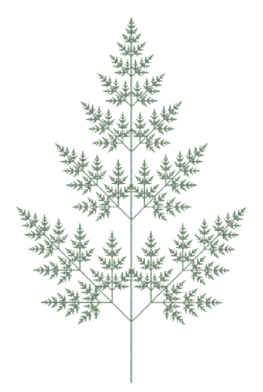 | 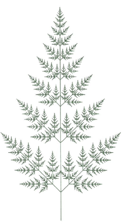 |  |  |
| b = 0 c = 2 Generations = 9 | b = 1 c = 0.5 Generations = 14 | b = 2 c = 1.36 Generations = 18 | b = 4 c = 1.23 Generations = 24 | b = 7 c = 1.17 Generations = 30 |
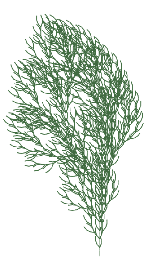
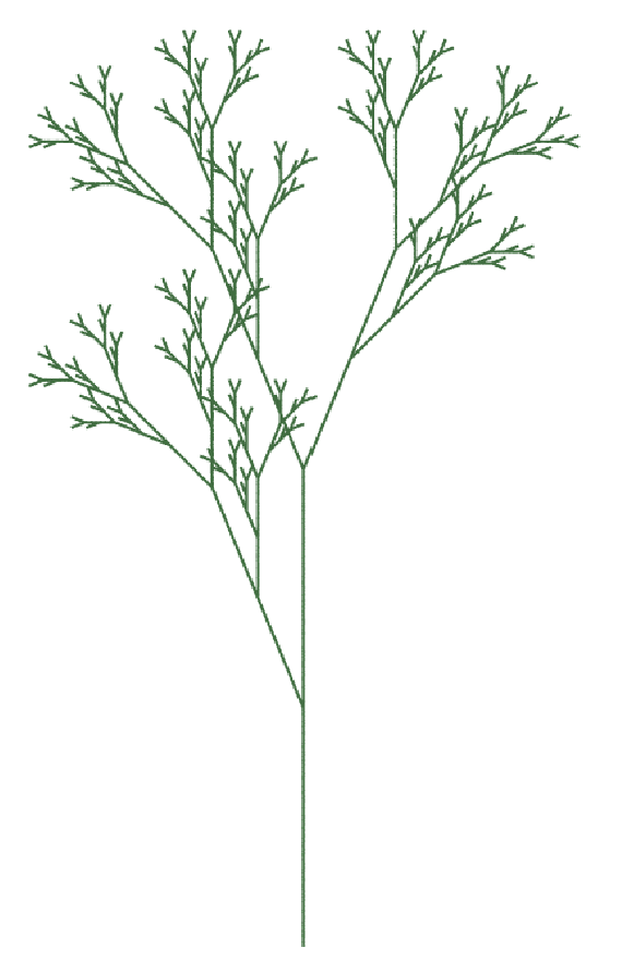
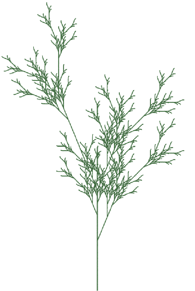
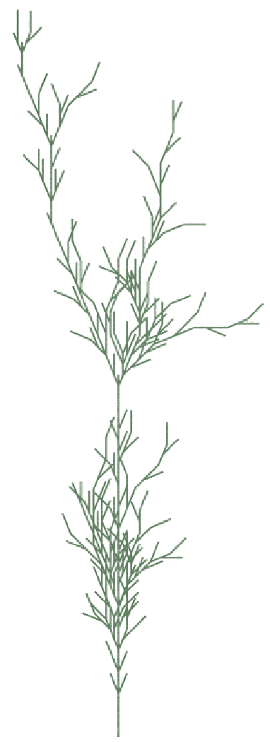
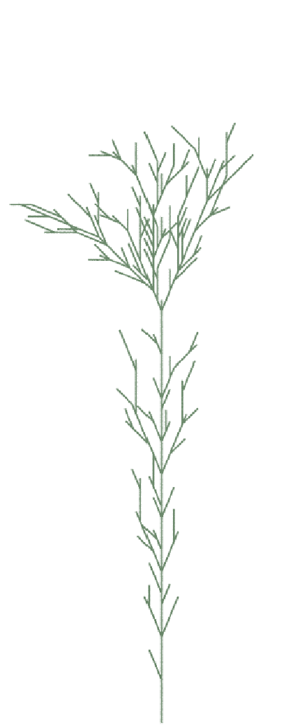
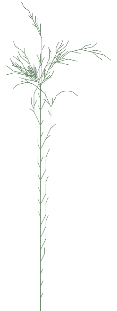
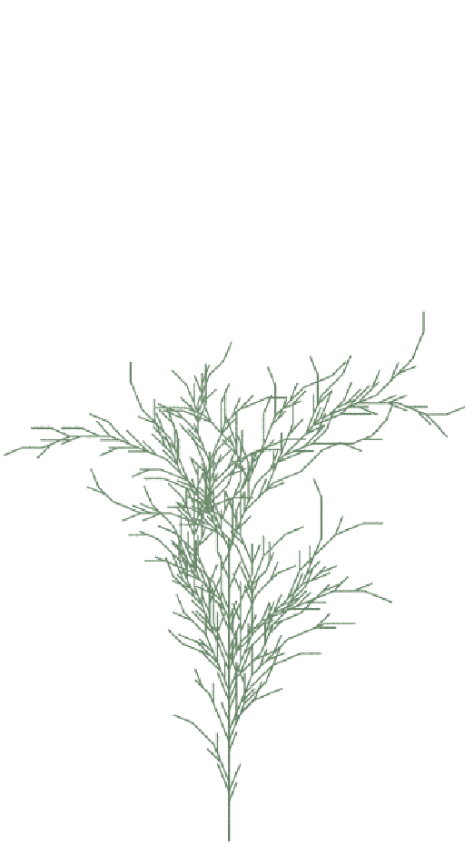
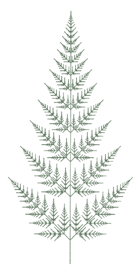
Compound leaves with alternating branching patterns
From The Algorithmic Beauty of Plants p.130, Figure 5.12
- b = apical delay (number of children on a frond, a whole number)
- c = internode elongation rate (decrease in size of fronds)
| Premise | A(0) |
| Rule 1 | A(i):i>0 = A(i-1) |
| Rule 2 | A(i):i=0 = F(1)[+A(b)]F(1)B(0) |
| Rule 3 | B(i):i>0 = B(i-1) |
| Rule 4 | B(i):i=0 = F(1)[-B(b)]F(1)A(0) |
| Rule 5 | F(a) = F(a*c) |
| Angle | 45 |
 | 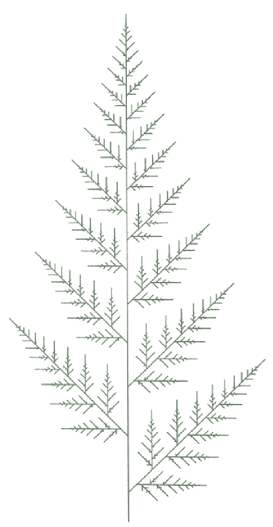 | 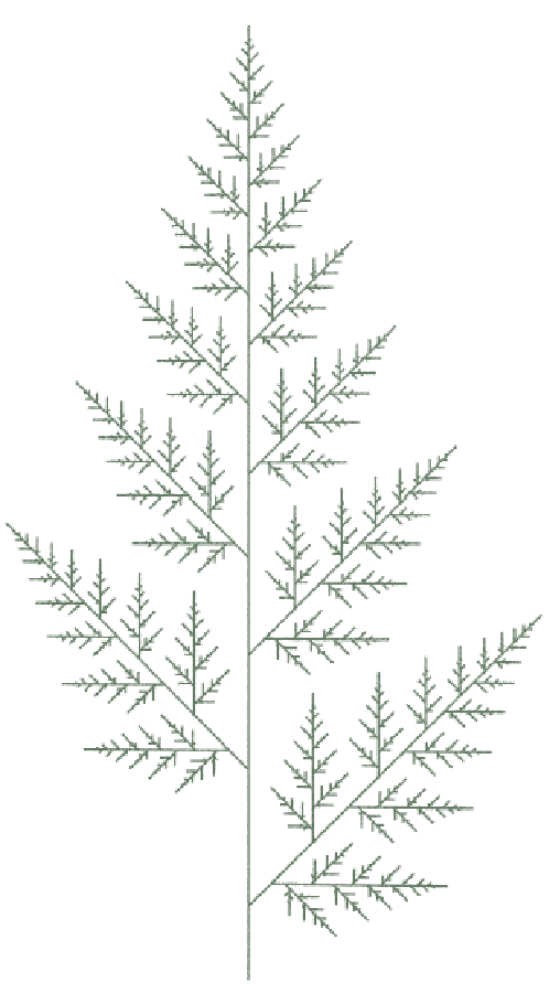 |
| b = 1 c = 1.36 Generations = 18 | b = 4 c = 1.18 Generations = 29 | b = 7 c = 1.13 Generations = 38 |
Leave a comment